Rides Time Series Prediction
- gracecamc168
- Dec 29, 2020
- 3 min read
Updated: Jan 7, 2021
This is one of the small project from one of my Business Analytics courses.
The dataset is from a software company in the Bay area, and I only use small part of it for this prediction. The purpose of this work is to compare different methods for this time series prediction. I will use Simple Moving Average(SMA) , Simple Exponential Smoothing(SES) and Linear Trend Model. We use R as the programming language for this project.
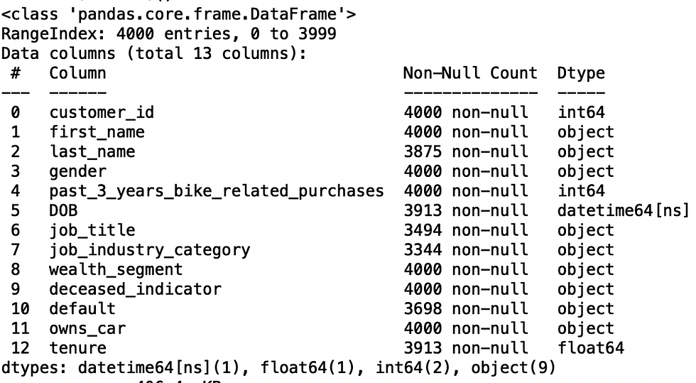
Let's glimpse the dataset. The observations are only from Mondays to Fridays.


We can see that there are missing values in the dataset.
The first thing I will do is to fill out the missing values because it is not that appropriate to leave missing values to do time series, and it might create computation error when we do performance measures such as MSE, MAD or MAPE. My Professor said it actually could leave them empty, but it is ok to fill it out with appropriate values. Therefore, I will fill them out.
The general method is to use the average value of all observations on Mondays to impute into the missing values of rides on Mondays and the average value of all observations on Tuesdays to impute the missing values of rides on Tuesday. Why only Mondays and Tuesdays? Because we only have missing values on these dates. Why only average value of Mondays or Tuesdays? Because rides are decreasing from Mondays to Fridays, meaning more people are taking rides on Mondays. It will mislead the trend if I use the value from averaging all the observations.
Let's see the graph.
There is clear seasonality with a weak upward movement trend

The reason I use SMA and SES for this case is just to justify why SMA and SES are not appropriate for trend and seasonality data, though SES could be used, it is still not that good.
The performance measures of MSE, MAD, MAPE for SMA are 113565.48,269.52, 10.3%, respectively.
The performance measures of MSE, MAD, MAPE for SES with the best alpha of 0.10531, which is generated by R, are 120191.321, 282.113,10.69% respectively.
The performance measures of MSE, MAD, MAPE for Linear trend model are 10041.61,76.33438,2.84%, respectively.
By the comparison of the performance measures, Linear model is clearly outperforming, because it generates much lower MSE, MAD, MAPE than other methods. Therefore, I choose Linear model for this time series prediction.
Let's visualize it. The linear model( red line) is much closer to the observed values than other methods.

Use the linear model for prediction
Before I conduct the model, I convert Monday,Tuesday, Wednesday,Thursday and Fridays into 1,2,3,4,5, and I create a new column for time (1:64).

The equation is rides = 2787.0163 + 3.8119 *d2 -148.6838*d3 -287.9488*d4 -843.4616*d5 + 7.7265*day, implying every day ,rides general increase by about 7.7 rides.
For this time series linear model, d1, meaning Monday, is the default factor in the model.The coefficients for the seasonal dummy variables indicate that, relative to Monday, the rides of Tuesday in general are higher than Monday by about 4 rides; Relative to Monday, the rides of Wednesday in general are lower than Monday by about 149 rides; Relative to Monday, the rides of Thursday in general are lower than Monday by about 288 rides; Relative to Monday, the rides of Friday in general are lower than Monday by about 843 rides. This model explains 91.84% of the sample variation in rides, remaining 8.16% unexplained, indicating high explanation power. The adjusted Rsquared, meaning after penalizing additional predictor in the model, is 91.13%, p-value is very small, nearly 0. Overall, this model looks good.
Based on this model, we can predict rides for all weekdays in April in 2016.

Visualization

I use the same strategy to predict the revenue for all weekdays in April of 2016.

Visualization


Comments