Quantium Retail Analytics Virtual Project
- gracecamc168
- Aug 6, 2021
- 17 min read
Updated: Sep 8, 2021
Background:
ABC company is interested in customer segments and their chip purchasing behaviors. Consider what metrics would help describe the customers’ purchasing behavior. In order to tackle the task, the company gave us two datasets--- transaction data and purchase behavior. I use both R and Python to accomplish this project. Python is for task one and R is for task two.
Purchase Behavior Dataset

Transaction Dataset
The original two datasets can be found here.
Task one: Purchasing behaviors
# import purchase_behaviour file
file = pd.read_csv("QVI_purchase_behaviour.csv")
file.info() # 72637 * 3
file.isnull().sum() # no missing value
file[file.duplicated()] # no duplication
# change the datatype for some columns
file['LYLTY_CARD_NBR'] = file['LYLTY_CARD_NBR'].astype(str)
# check for groups for columns
file['LIFESTAGE'].value_counts()
file['PREMIUM_CUSTOMER'].value_counts()
# change the name for columns
file = file.rename(columns=str.lower)
# import transaction file
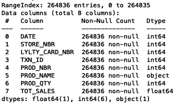
trans = pd.read_excel("QVI_transaction_data.xlsx")
trans.info() # 264836 * 8
trans.isnull().sum() # no missing value
trans[trans.duplicated()] # 1 duplication, drop it
trans = trans.drop_duplicates()
# change column name to lowercase
trans = trans.rename(columns=str.lower)
# change datatype, and date format
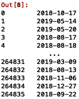
date_offsets = trans['date']
base_date = pd.Timestamp('1899-12-30')
dates = [
base_date + pd.DateOffset(date_offset)
for date_offset in date_offsets
]
print(dates[0:5])
trans['date'] = pd.to_datetime(dates)
# change other datatypes
trans['store_nbr'] = trans['store_nbr'].astype(str)
trans['lylty_card_nbr'] = trans['lylty_card_nbr'].astype(str)
trans['txn_id'] = trans['txn_id'].astype(str)
trans['prod_nbr'] = trans['prod_nbr'].astype(str)
trans['prod_nbr'] = trans['prod_nbr'].astype(str)
# extract weight(digits) from prod_name column
trans['weight_g'] = trans['prod_name'].str.extract('(\d+)')
trans['weight_g'] = trans['weight_g'].astype(int)
trans['weight_g'].value_counts()
# remove weight from prod_name column
trans['prod_name'] = trans['prod_name'].str[:-3]
trans['prod_name'] = trans['prod_name'].str[:-1]
'''
prod_name column
'''
# remove double/mutiple space between words from prod_name column
pd.set_option('max_columns', 200)
pd.set_option('max_rows', 200)
trans['prod_name'] = trans['prod_name'].replace('\s+', ' ', regex=True)
unique_value = trans['prod_name'].value_counts() # 114
# remove space aside &
trans['prod_name'] = trans['prod_name'].str.replace(" & ", "&")
trans['prod_name'].value_counts()
# change the value name
trans['prod_name'] = trans['prod_name'].str.replace("Vinegr","Vinegar")
'''
brand name and flavor from prod_name column
'''
# extract the brand name
trans['brand_name'] = trans['prod_name'].str.split().str[0]
trans['brand_name'].value_counts()
# correct the brand name value
trans['brand_name'] = trans['brand_name'].str.replace("RRD","Red Rock Deli")
trans['brand_name'] = trans['brand_name'].str.replace("Old","Old El Paso")
trans['brand_name'] = trans['brand_name'].str.replace("Grain","Grain Waves")
trans['brand_name'] = trans['brand_name'].str.replace("Red","Red Rock Deli")
trans['brand_name'] = trans['brand_name'].str.replace("Dorito","Doritos")
trans['brand_name'] = trans['brand_name'].str.replace("Infzns","Infuzions")
trans['brand_name'] = trans['brand_name'].str.replace("Smith","Smiths")
trans['brand_name'] = trans['brand_name'].str.replace("GrnWves","Grain Waves")
trans['brand_name'] = trans['brand_name'].str.replace("Snbts","Sunbites")
trans['brand_name'] = trans['brand_name'].str.replace("NCC","Natural")
trans['brand_name'] = trans['brand_name'].str.replace("RRD","Red Rock Deli")
trans['brand_name'].value_counts()
trans['brand_name'] = trans['brand_name'].str.replace("Red Rock Deli Rock Deli","Red Rock Deli")
trans['brand_name'] = trans['brand_name'].str.replace("Smithss","Smiths")
trans['brand_name'] = trans['brand_name'].str.replace("Doritoss","Doritos")
# extract the flavor
trans['flavor'] = trans['prod_name'].str.split().str[-2:].str.join(' ')
trans['flavor'].value_counts()
# correct the flavor name value
trans['flavor'] = trans['flavor'].str.replace("Pot Sea","SwtPot Sea")
trans['flavor'] = trans['flavor'].str.replace("Of Lime","Lime")
trans['flavor'] = trans['flavor'].str.replace("And Vinegar","Salt&Vinegar")
trans['flavor'] = trans['flavor'].str.replace("Kettle Chilli","Chilli")
trans['flavor'] = trans['flavor'].str.replace("N Cheese ","Cheese")
trans['flavor'] = trans['flavor'].str.replace("Soy Chckn","Soy Chicken")
trans['flavor'] = trans['flavor'].str.replace("Compny SeaSalt","SeaSalt")
trans['flavor'] = trans['flavor'].str.replace("Compny SeaSalt","SeaSalt")
trans['flavor'] = trans['flavor'].str.replace("Chips Salt&Vinegar","Salt&Vinegar")
trans['flavor'] = trans['flavor'].str.replace("Cut Original","Original")
trans['flavor'] = trans['flavor'].str.replace("Slt Vingar","Salt&Vinegar")
trans['flavor'] = trans['flavor'].str.replace("CCs Original","Original")
trans['flavor'] = trans['flavor'].str.replace("Chips Original","Original")
trans['flavor'] = trans['flavor'].str.replace("Kettle Original","Original")
trans['flavor'] = trans['flavor'].str.replace("Original Crisps","Original")
trans['flavor'] = trans['flavor'].str.replace("Crinkle Original","Original")
trans['flavor'] = trans['flavor'].str.replace("RRD Salt&Vinegar","Salt&Vinegar")
trans['flavor'] = trans['flavor'].str.replace("Cut Salt&Vinegar","Salt&Vinegar")
trans['flavor'] = trans['flavor'].str.replace("Cheese Supreme","Cheese")
trans['flavor'] = trans['flavor'].str.replace("Cheezels Cheese","Cheese")
trans['flavor'] = trans['flavor'].str.replace("Twisties Cheese","Cheese")
trans['flavor'] = trans['flavor'].str.replace("Tasty Cheese","Cheese")
trans['flavor'] = trans['flavor'].str.replace("N Cheese","Cheese")
trans['flavor'] = trans['flavor'].str.replace("Cheese Box","Cheese")
trans['flavor'] = trans['flavor'].str.replace("Cheese Rings","Cheese")
trans['flavor'] = trans['flavor'].str.replace("Twisties Chicken","Chicken")
trans['flavor'] = trans['flavor'].str.replace("Chips Chicken","Chicken")
trans['flavor'] = trans['flavor'].str.replace("Cut Chicken","Chicken")
trans['flavor'] = trans['flavor'].str.replace("Salsa Mild","Mild Salsa")
trans['flavor'] = trans['flavor'].str.replace("Salsa Medium","Medium Salsa")
trans['flavor'] = trans['flavor'].str.replace("Chp Supreme","Cheese")
trans['flavor'] = trans['flavor'].str.replace("Doritos Mexicana","Mexicana")
# recheck the dataframe
trans.info()
# find out the rows only contain chips from the product name column
chips = trans[trans['prod_name'].str.contains("Chip")]
# check if there is duplication
chips[chips.duplicated()] # no duplication
chips.info()
# create a column containing the month
chips['month'] = pd.to_datetime(chips['date']).dt.to_period('M')
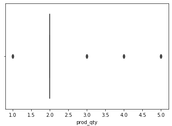
# any outliers?
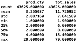
chips['prod_qty'].describe()
sns.boxplot(x=chips['prod_qty'])
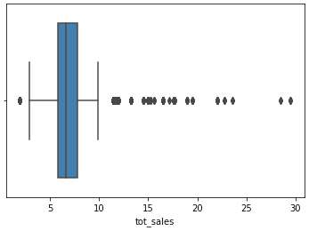
chips['tot_sales'].describe()
sns.boxplot(x=chips['tot_sales'])
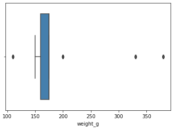
chips['weight_g'].describe()
sns.boxplot(x=chips['weight_g'])
# yes, outliers
# groupby loyal customers to check if there are outliers?
aggreation = pd.DataFrame(chips.groupby(['lylty_card_nbr'],as_index=False).agg({'prod_qty':'sum',
'tot_sales':'sum'}))
aggreation.sort_values('tot_sales', ascending=False).head()
aggreation.describe()
# it looks like outliers, but we keep all the data by now
# count the number of transactions per day
pd.set_option('max_columns', 200)
pd.set_option('max_rows', 200)
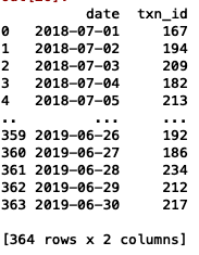
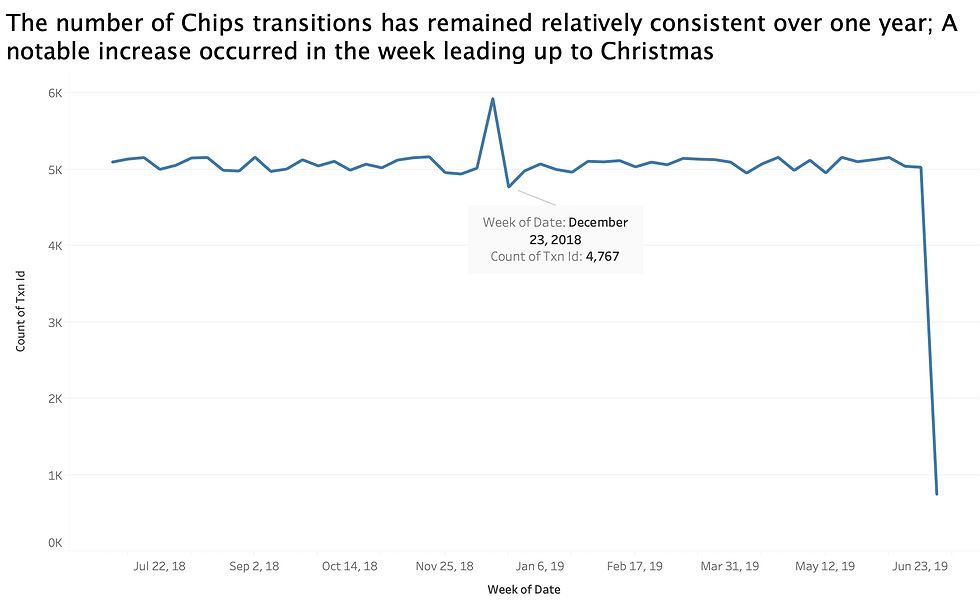
total_trans = pd.DataFrame(chips.groupby(['date'],as_index=False).agg({'txn_id':'count'}))
# 364 dates, meaning there is a missing date
# create a line chart
plt.figure(figsize=(12, 12), dpi=80)
plt.plot(total_trans['date'],total_trans['txn_id'], color='red', marker='o')
plt.title('Transactions per day', fontsize=14)
plt.xlabel('Date', fontsize=14)
plt.ylabel('Counts', fontsize=14)
plt.grid(True)
plt.show()
# we can see that 2018-12-25 did not have any transactions, the stores might be closed for Christmas.
# combine two datasets together based on card number, but taking all the rows in the transaction table
new_file = chips.merge(file,on='lylty_card_nbr',how='left')
new_file.info()
# check if there is duplication
new_file[new_file.duplicated()] # no duplication
new_file.isnull().sum() # no missing values
# calcuate the average price for each segment of lifestage and premium customer
avg_price = pd.DataFrame(new_file.groupby(['premium_customer','lifestage'],as_index=False).agg({'tot_sales':'sum','prod_qty':'sum'}))
avg_price['mean_price'] = avg_price['tot_sales'] / avg_price['prod_qty']
plt.figure(figsize=(8, 8), dpi=80)
sns.barplot(y='mean_price',x='premium_customer',hue='lifestage',data=avg_price)
plt.legend(loc='top left')
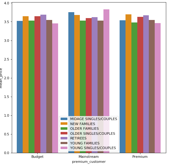
# it seems that Mainstream midage and young singles and couples are more willing to pay
# more per packet of chips compared to their budget and premium counterparts.
# since the difference in average price per unit is not huge, we can check if
# the difference is statistically different?
'''
T test
'''
# conduct a T test for mainstream's young singles/couples and budget's young singles/couples,
# mainstream's mid singles/couples and budget's mid singles/couples,
# mainstream's mid singles/couples and premium's mid singles/couples,
# mainstream's young singles/couples and premium's young singles/couples
# subset the relevant columns
testing = new_file[['premium_customer','lifestage','prod_qty','tot_sales']]
testing['mean_price'] = testing['tot_sales'] / avg_price['prod_qty']
# subset the relevant columns
testing1 = testing[['premium_customer','lifestage','mean_price']]
from scipy import stats
# this is for mainstream's young singles/couples and premium's young singles/couples
sample_1 = testing1.query('premium_customer == "Premium" & lifestage == "YOUNG SINGLES/COUPLES"')
sample_2 = testing1.query('premium_customer == "Mainstream" & lifestage == "YOUNG SINGLES/COUPLES"')
t_result = stats.ttest_ind(sample_1['mean_price'],sample_2['mean_price'])
alpha = 0.05
if (t_result[1]) < alpha:
print("mainstream's young singles/couples and premium's young singles/couples are significantly different,the T value is",
t_result[1])
else:
print("Not significantly different")
# the T value is 1.14064138830466e-49
# this is for mainstream's mid singles/couples and premium's mid singles/couples
sample_1 = testing1.query('premium_customer == "Premium" & lifestage == "MIDAGE SINGLES/COUPLES"')
sample_2 = testing1.query('premium_customer == "Mainstream" & lifestage == "MIDAGE SINGLES/COUPLES"')
t_result = stats.ttest_ind(sample_1['mean_price'],sample_2['mean_price'])
alpha = 0.05
if (t_result[1]) < alpha:
print("mainstream's mid singles/couples and premium's mid singles/couples are significantly different,the T value is",
t_result[1])
else:
print("Not significantly different")
# the T value is 5.584689508431946e-17
# this is for mainstream's young singles/couples and budget's young singles/couples
sample_1 = testing1.query('premium_customer == "Budget" & lifestage == "YOUNG SINGLES/COUPLES"')
sample_2 = testing1.query('premium_customer == "Mainstream" & lifestage == "YOUNG SINGLES/COUPLES"')
t_result = stats.ttest_ind(sample_1['mean_price'],sample_2['mean_price'])
alpha = 0.05
if (t_result[1]) < alpha:
print("mainstream's young singles/couples and budget's young singles/couples are significantly different,the T value is",
t_result[1])
else:
print("Not significantly different")
# the T value is 6.273067126806781e-68
# this is for mainstream's mid singles/couples and budget's mid singles/couples
sample_1 = testing1.query('premium_customer == "Budget" & lifestage == "MIDAGE SINGLES/COUPLES"')
sample_2 = testing1.query('premium_customer == "Mainstream" & lifestage == "MIDAGE SINGLES/COUPLES"')
t_result = stats.ttest_ind(sample_1['mean_price'],sample_2['mean_price'])
alpha = 0.05
if (t_result[1]) < alpha:
print("mainstream's mid singles/couples and budget's mid singles/couples are significantly different,the T value is",
t_result[1])
else:
print("Not significantly different")
# the T value is 3.605581037486487e-15
Results:
All tests above show that the unit price for mainstream, young and mid-age singles and couples are significantly higher than that of budget or premium, young and midage singles and couples.
Visualization
Now we have cleaned and conducted some analysis to our datasets. Let's explore the data to discover the behaviors of each segment. I use Tableau for this task.
Summary Statistic
There is a total of 8 brands, 29 flavors in chips category. The top 3 brands based on sales are Smiths, Doritos, Thins, their sales in total are accounted for 67.57% of the whole sales. These brands have the highest number of flavors as well.
There are 43625 loyal customers; 265 number of stores.
Cheese, original, salt vinegar are the top 3 flavors among all the customer groups(lifestages, premium customer groups)
Finding 1:

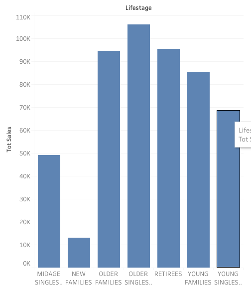
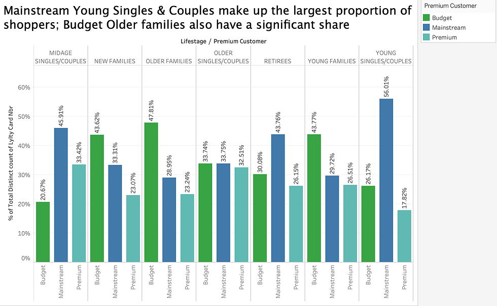
Mainstream customers purchase the most, while premium customers are the lowest. It might be because wealthy customer can afford other more expensive snacks/food.
Older singles/couples purchase the most. In general, older people purchase more than younger people, it could be partly because older people have less other social events but young people
have a lot more. Therefore, older people stay at home more, they have time to eat chips while watching TV. New families group purchase the least, it is likely that they need to keep their life healthy or simply they don’t have much spare time to chill at home because they need to raise their kids.
Finding 2:
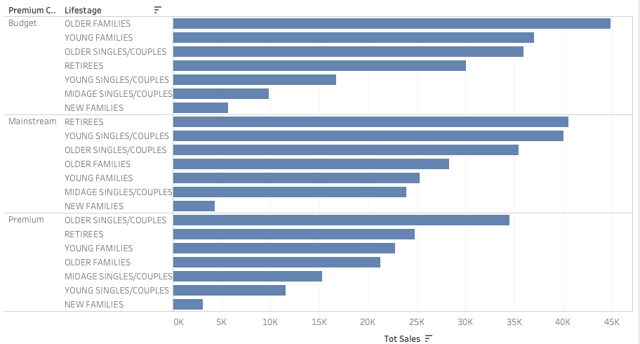
Families tend to be budget customers. Perhaps they need money to raise the kids, so they don’t have much money on snacks.
Finding 3:
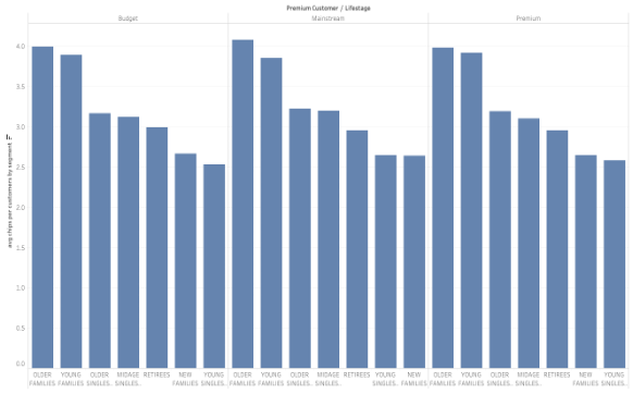
Average chips purchased by each customer by lifestage and premium customer. It seems that older families and young families of each customer segment consume more average chips than other segments.
Finding 4:
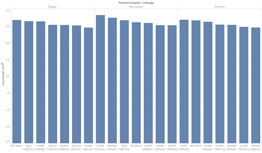
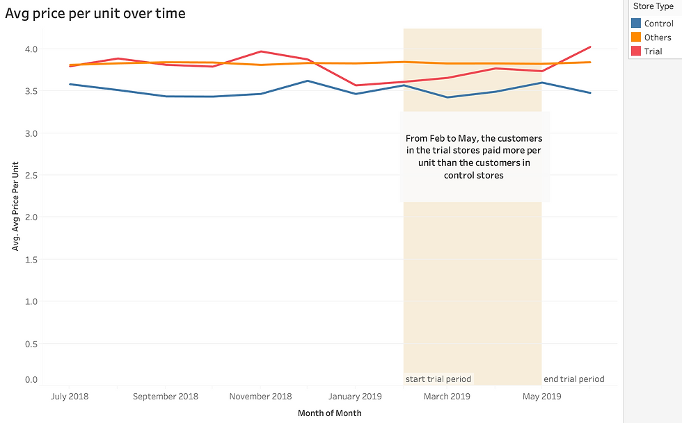
Average price per unit by lifestage and premium customer. It seems that Mainstream midage and young singles and couples are more willing to pay more per bag of chips compared to their budget and premium counterparts. Since the difference in average price per unit is not huge, I checked if the difference is statistically different. The result conducted by T test in python showed that the unit price for mainstream, young and mid-age singles and couples ARE significantly higher than that of budget or premium, young and midage singles and couples.
Finding 5:
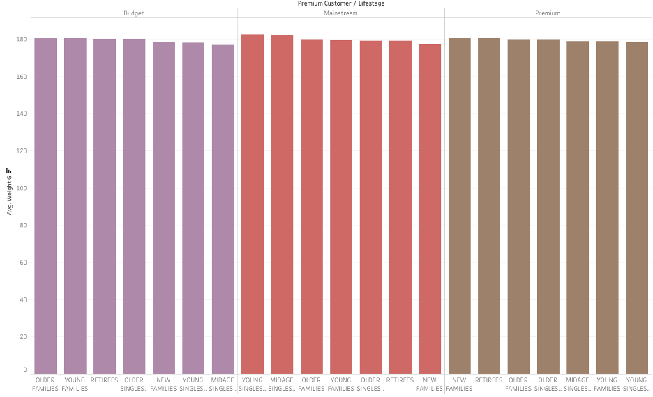
On average, it seems that customers from each segment like regular size of package 180.
Based upon the visualizations above, we should set our target customers to be Budget’s older families, Mainstream’s retires or young singles/couples.
Now that we identified the target segments. We are also interested in whether the target segments have any preferences toward such as favors, package size and brands etc. To do so, we use brand affinity analysis. Let's only consider Mainstream’s young singles/couples as the target segment by now.
## brand affinity
# subset the data into only contain Mainstream’s young singles/couples
sample = new_file.query('premium_customer == "Mainstream" & lifestage == "YOUNG SINGLES/COUPLES"')
# sum the quantity of Mainstream’s young singles/couples
segment_quantity = sum(sample['prod_qty']) # 10459
# find out the brands of the sample data subset
sample['brand_name'].value_counts()
# sum the quantity by each brand
brand_quantity = pd.DataFrame(sample.groupby(['brand_name'],as_index=False).agg({'prod_qty':'sum'}))
# divide by segment_quantity
quantity_segment_by_brand = pd.DataFrame(brand_quantity['prod_qty'] / segment_quantity)
# add column name
quantity_segment_by_brand.rename({'prod_qty': 'target'}, axis=1, inplace=True)
# put it back to the dataset
target_quantity_brand = pd.concat([brand_quantity, quantity_segment_by_brand], axis=1)
# sum other segments' quantity
sample_other = new_file.query('premium_customer != "Mainstream" & lifestage != "YOUNG SINGLES/COUPLES"')
total_quantity = sum(sample_other['prod_qty']) # 79504
# find out the brands of the sample data subset
sample_other['brand_name'].value_counts()
# sum the quantity by each brand
brand_other_quantity = pd.DataFrame(sample_other.groupby(['brand_name'],as_index=False).agg({'prod_qty':'sum'}))
# divide by segment_quantity
quantity_other_by_brand = pd.DataFrame(brand_other_quantity['prod_qty'] / total_quantity)
# add column name
quantity_other_by_brand.rename({'prod_qty': 'others'}, axis=1, inplace=True)
# put it back to the dataset
other_quantity_brand = pd.concat([brand_other_quantity, quantity_other_by_brand], axis=1)
other_quantity_brand.sort_values('others', ascending=False)
# merge two datasets
total = pd.DataFrame(other_quantity_brand.merge(target_quantity_brand,on='brand_name',how='inner'))
# only keep few columns
total = total.drop(['prod_qty_x','prod_qty_y'],axis=1)
# get the affiniity to brand
total['affinityToBrand'] = pd.DataFrame(total.target / total.others)
# sort the value by affinityToBrand
total.sort_values('affinityToBrand', ascending=False)
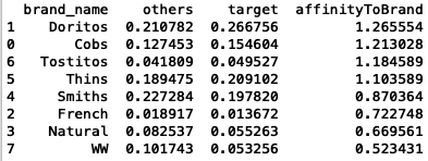
Results:
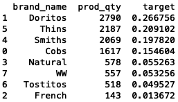
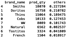
Mainstream young singles/couples are 26% more likely to purchase Doritos chips compared to the rest of the population.
Mainstream's young singles/couples are 48% less likely to purchase WW compared to the rest of the population.
## repeat the steps to calculate the package size
# sum the quantity of Mainstream’s young singles/couples
segment_quantity = sum(sample['prod_qty']) # 10459
# find out the brands of the sample data subset
sample['weight_g'].value_counts()
# sum the quantity by each brand
weight_quantity = pd.DataFrame(sample.groupby(['weight_g'],as_index=False).agg({'prod_qty':'sum'}))
# divide by segment_quantity
weight_segment_by_brand = pd.DataFrame(weight_quantity['prod_qty'] / segment_quantity)
# add column name
weight_segment_by_brand.rename({'prod_qty': 'target'}, axis=1, inplace=True)
# put it back to the dataset
target_weight = pd.concat([weight_quantity, weight_segment_by_brand], axis=1)
target_weight.sort_values('target', ascending=False)
# sum other segments' quantity
sample_other = new_file.query('premium_customer != "Mainstream" & lifestage != "YOUNG SINGLES/COUPLES"')
total_quantity = sum(sample_other['prod_qty']) # 79504
# find out the brands of the sample data subset
sample_other['weight_g'].value_counts()
# sum the quantity by each brand
weight_other_quantity = pd.DataFrame(sample_other.groupby(['weight_g'],as_index=False).agg({'prod_qty':'sum'}))
# divide by segment_quantity
weight_others = pd.DataFrame(weight_other_quantity['prod_qty'] / total_quantity)
# add column name
weight_others.rename({'prod_qty': 'others'}, axis=1, inplace=True)
# put it back to the dataset
other_quantity_weight = pd.concat([weight_other_quantity, weight_others], axis=1)
other_quantity_weight.sort_values('others', ascending=False)
# merge two datasets
weights = pd.DataFrame(other_quantity_weight.merge(target_weight,on='weight_g',how='inner'))
# only keep few columns
weights = weights.drop(['prod_qty_x','prod_qty_y'],axis=1)
# get the affiniity to weight
weights['affinityToWeight'] = pd.DataFrame(weights.target / weights.others)
# sort the value by affinityToWeight
weights.sort_values('affinityToWeight', ascending=False)
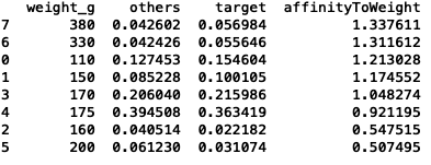
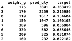
Results:
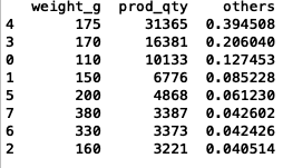
Mainstream young singles/couples are 34% more likely to purchase 380 package size compared to the rest of the population.
Mainstream young singles/couples are 50% less likely to purchase 200 package size compared to the rest of the population
## repeat the steps to calculate the flavor
# sum the quantity of Mainstream’s young singles/couples
segment_quantity = sum(sample['prod_qty']) # 10459
# find out the brands of the sample data subset
sample['flavor'].value_counts()
# sum the quantity by each brand
flavor_quantity = pd.DataFrame(sample.groupby(['flavor'],as_index=False).agg({'prod_qty':'sum'}))
# divide by segment_quantity
flavor_segment_by_brand = pd.DataFrame(flavor_quantity['prod_qty'] / segment_quantity)
# add column name
flavor_segment_by_brand.rename({'prod_qty': 'target'}, axis=1, inplace=True)
# put it back to the dataset
target_flavor = pd.concat([flavor_quantity,flavor_segment_by_brand], axis=1)
target_flavor.sort_values('target', ascending=False)
# sum other segments' quantity
sample_other = new_file.query('premium_customer != "Mainstream" & lifestage != "YOUNG SINGLES/COUPLES"')
total_quantity = sum(sample_other['prod_qty']) # 79504
# find out the brands of the sample data subset
sample_other['flavor'].value_counts()
# sum the quantity by each brand
flavor_other_quantity = pd.DataFrame(sample_other.groupby(['flavor'],as_index=False).agg({'prod_qty':'sum'}))
# divide by segment_quantity
flavor_others = pd.DataFrame(flavor_other_quantity['prod_qty'] / total_quantity)
# add column name
flavor_others.rename({'prod_qty': 'others'}, axis=1, inplace=True)
# put it back to the dataset
other_quantity_flavor = pd.concat([flavor_other_quantity,flavor_others], axis=1)
# merge two datasets
flavors = pd.DataFrame(other_quantity_flavor.merge(target_flavor,on='flavor',how='inner'))
# only keep few columns
flavors = flavors.drop(['prod_qty_x','prod_qty_y'],axis=1)
# get the affiniity to brand
flavors['affinityToBrand'] = pd.DataFrame(flavors.target / flavors.others)
# sort the value by affinityToBrand
flavors.sort_values('affinityToBrand', ascending=False)
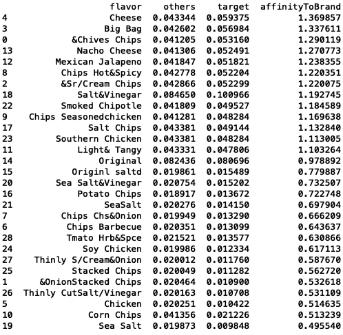
Results:
Mainstream young singles/couples are 37% more likely to purchase cheese compared to
the rest of the population.
Mainstream young singles/couples are 51% less likely to purchase sea salt compared to the rest of the population.
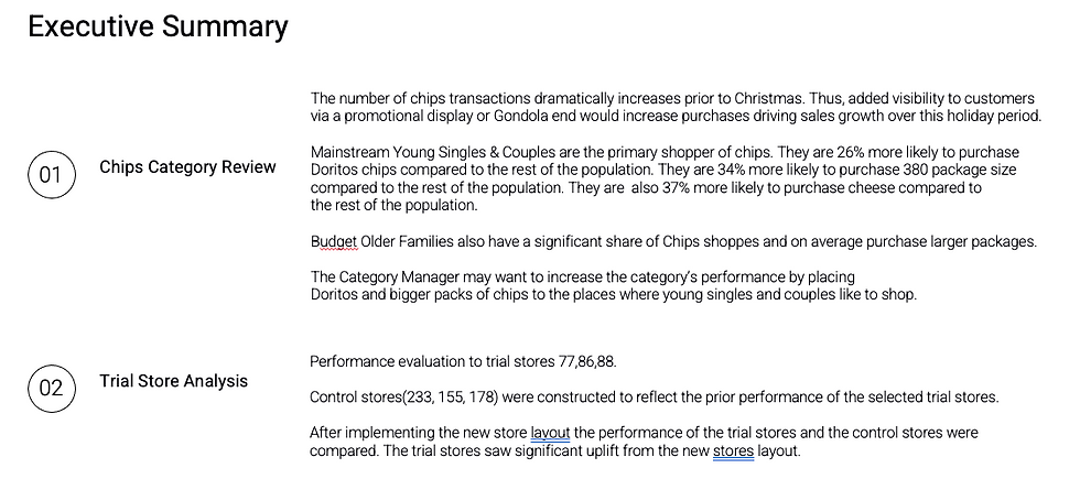
Conclusion
Sales are mainly from Mainstream's young singles/couples and Mainstream's retirees shoppers.
The high spend in chips for mainstream young singles/couples and retirees is due to there being more of them than other buyers.
Mainstream, midage and young singles and couples are also more likely to pay more
per packet of chips. We’ve also found that Mainstream young singles and couples
are 26% more likely to purchase Doritos chips compared to the rest of the population.
Mainstream young singles and couples are also 34% more likely to purchase 380 package size compared to the rest of the population.
Mainstream young singles/couples are 37% more likely to purchase cheese compared to
the rest of the population.
The Category Manager may want to increase the category’s performance by placing
Doritos and bigger packs of chips to the places where young singles and couples like to shop.
Task two: Evaluating the performance of a store trial which was performed in stores 77, 86 and 88.
To get started use the QVI_data dataset below(the output from task 1) and consider the monthly sales experience of each store.
This can be broken down by:
total sales revenue
total number of customers
average number of transactions per customer
Create a measure to compare different control stores to each of the trial stores to do this write a function to reduce having to redo the analysis for each trial store. Consider using Pearson correlations or a metric such as a magnitude distance e.g. 1- (Observed distance – minimum distance)/(Maximum distance – minimum distance) as a measure.
Once we have selected the control stores, compare each trial and control pair during the trial period. We want to test if total sales are significantly different in the trial period and if so, check if the driver of change is more purchasing customers or more purchases per customers etc.
# read the file
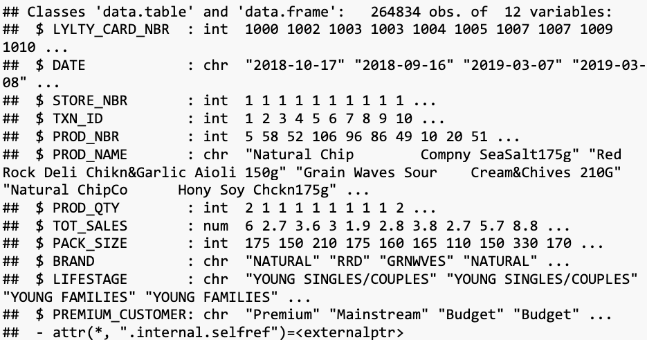
data <- fread("QVI_data.csv")
str(data)
# set themes for plots
theme_set(theme_bw()) theme_update(plot.title = element_text(hjust = 0.5))
# add a new month ID column in the data with the format yyyymm
class(data$YEARMONTH)
## [1] "NULL"
data$YEARMONTH <- as.numeric(monthYear)
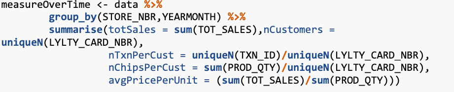
Next, we define the measure calculations to use during the analysis. For each store and month calculate total sales, number of customers, transactions per customer, chips per customer and the average price per unit.
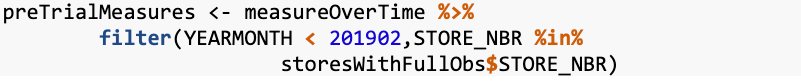
# filter to the pre-trial period and stores with 12-month periods stores with a 12-month period
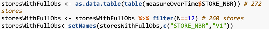
# Filter to the pre-trial period
Now we need to work out a way of ranking how similar each potential control store is to the trial store. We can calculate how correlated the performance of each store is to the trial store.
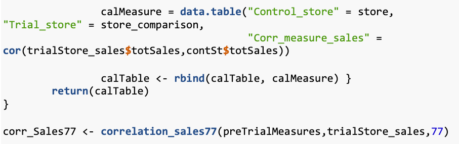
# Sales for trial store 77
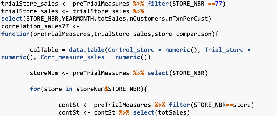
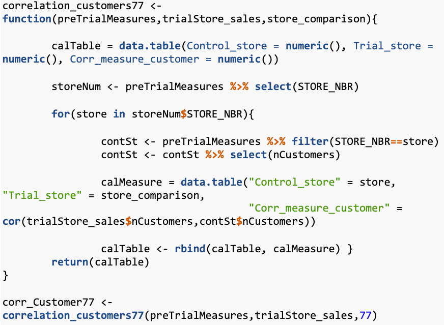
# Customers for trial store 77
# number of transactions per customer for trial store 77
correlation_nTxnPerCust77 <- function(preTrialMeasures,trialStore_sales,store_comparison){
calTable = data.table(Control_store = numeric(), Trial_store = numeric(), Corr_measure_nTxnPerCust = numeric())
storeNum <- preTrialMeasures %>% select(STORE_NBR)
for(store in storeNum$STORE_NBR){
contSt <- preTrialMeasures %>% filter(STORE_NBR==store)
contSt <- contSt %>% select(nTxnPerCust)
calMeasure = data.table("Control_store" = store, "Trial_store" = store_comparison,
"Corr_measure_nTxnPerCust" = cor(trialStore_sales$nTxnPerCust,contSt$nTxnPerCust))
calTable <- rbind(calTable, calMeasure) }
return(calTable)
}
corr_nTxnPerCust77 <- correlation_nTxnPerCust77(preTrialMeasures,trialStore_sales,77)
### Apart from correlation, we can also calculate a standardised metric based on the
### absolute difference between the trial store's performance and each control store's
### performance.
#### Create a function to calculate a standardised magnitude distance for a measure, looping ### through each control store
### Sales
calculateMagnitudeDistance <- function(preTrialMeasures,trialStore_sales,storeComparison){
calTable = data.table(Control_store = numeric(), Trial_store = numeric(),
YEARMONTH = numeric(),mag_measure = numeric())
storeNumbers <- preTrialMeasures %>% select(STORE_NBR)
for(store in storeNumbers$STORE_NBR){
contSt <- preTrialMeasures %>% filter(STORE_NBR==store)
contSt <- contSt %>% select(totSales)
calMeasure = data.table("Control_store" = store, "Trial_store" = storeComparison,
"YEARMONTH" = preTrialMeasures$YEARMONTH ,
"mag_measure" = abs(trialStore_sales$totSales - contSt$totSales))
calTable <- rbind(calTable,calMeasure)
calTable <- unique(calTable)
}
return(calTable)
}
calculateMagnitudeDistanceSales <- calculateMagnitudeDistance(preTrialMeasures, trialStore_sales, 77)
#### Standardise the magnitude distance so that the measure ranges from 0 to 1
standMagSales <- function(magnitude_nSales) {
minMaxDist <- magnitude_nSales[, .(minDist = min( magnitude_nSales$mag_measure),
maxDist = max(magnitude_nSales$mag_measure)),
by = c("Control_store", "YEARMONTH")]
distTable <- merge(magnitude_nSales, minMaxDist, by = c("Control_store", "YEARMONTH"))
distTable$magnitudeMeasure = 1 - (distTable$mag_measure - distTable$minDist)/(distTable$maxDist - distTable$minDist)
finalDistTable <- distTable[, .(magN_mean_measure = mean(magnitudeMeasure)), by = c("Control_store", "Trial_store")]
return(finalDistTable)
}
magnitude_nSales <- calculateMagnitudeDistance(preTrialMeasures, trialStore_sales, 77)
magnitude_nSales1 <- standMagSales(magnitude_nSales)
## For Customers
calculateMagnitudeDistance2 <- function(preTrialMeasures,trialStore_sales,storeComparison){
calTable = data.table(Control_store = numeric(), Trial_store = numeric(),
YEARMONTH = numeric(),mag_measure = numeric())
storeNumbers <- preTrialMeasures %>% select(STORE_NBR)
for(store in storeNumbers$STORE_NBR){
contSt <- preTrialMeasures %>% filter(STORE_NBR==store)
contSt <- contSt %>% select(nCustomers)
calMeasure = data.table("Control_store" = store, "Trial_store" = storeComparison,
"YEARMONTH" = preTrialMeasures$YEARMONTH ,
"mag_measure" = abs(trialStore_sales$nCustomers - contSt$nCustomers))
calTable <- rbind(calTable,calMeasure)
calTable <- unique(calTable)
}
return(calTable)
}
calculateMagnitudeDistanceCustomers <- calculateMagnitudeDistance2(preTrialMeasures, trialStore_sales, 77)
### Standardize
standMagCustomer <- function(magnitude_nCustomers) {
minMaxDist <- magnitude_nCustomers[, .(minDist = min(magnitude_nCustomers$mag_measure),
maxDist = max(magnitude_nCustomers$mag_measure)),
by = c("Control_store", "YEARMONTH")]
distTable <- merge(magnitude_nCustomers, minMaxDist, by = c("Control_store", "YEARMONTH"))
distTable$magnitudeMeasure <- 1 - (distTable$mag_measure - distTable$minDist)/(distTable$maxDist - distTable$minDist)
finalDistTable <- distTable[, .(magN_mean_measure = mean(magnitudeMeasure)), by = c("Control_store", "Trial_store")]
return(finalDistTable)
}
magnitude_nCustomers <- calculateMagnitudeDistance(preTrialMeasures, trialStore_sales, 77)
magnitude_nCustomer <- standMagCustomer(magnitude_nCustomers)
### For number of transactions per customer for trial store 77
calculateMagnitudeDistance3 <- function(preTrialMeasures,trialStore_sales,storeComparison){
calTable = data.table(Control_store = numeric(), Trial_store = numeric(),
YEARMONTH = numeric(),mag_measure = numeric())
storeNumbers <- preTrialMeasures %>% select(STORE_NBR)
for(store in storeNumbers$STORE_NBR){
contSt <- preTrialMeasures %>% filter(STORE_NBR==store)
contSt <- contSt %>% select(nTxnPerCust)
calMeasure = data.table("Control_store" = store, "Trial_store" = storeComparison,
"YEARMONTH" = preTrialMeasures$YEARMONTH ,
"mag_measure" = abs(trialStore_sales$nTxnPerCust - contSt$nTxnPerCust))
calTable <- rbind(calTable,calMeasure)
calTable <- unique(calTable)
}
return(calTable)
}
calculateMagnitudeDistancenTxnPerCust <- calculateMagnitudeDistance3(preTrialMeasures, trialStore_sales, 77)
### Standardize
standMagnTxnPerCust <- function(magnitude_nTxnPerCust) {
minMaxDist <- magnitude_nTxnPerCust[, .(minDist = min(magnitude_nTxnPerCust$mag_measure),
maxDist = max(magnitude_nTxnPerCust$mag_measure)),
by = c("Control_store", "YEARMONTH")]
distTable <- merge(magnitude_nCustomers, minMaxDist, by = c("Control_store", "YEARMONTH"))
distTable$magnitudeMeasure <- 1 - (distTable$mag_measure - distTable$minDist)/(distTable$maxDist - distTable$minDist)
finalDistTable <- distTable[, .(magN_mean_measure = mean(magnitudeMeasure)), by = c("Control_store", "YEARMONTH")]
return(finalDistTable)
}
magnitude_nTxnPerCust <- calculateMagnitudeDistance(preTrialMeasures, trialStore_sales, 77)
magnitudenTxnPerCust <- standMagnTxnPerCust(magnitude_nTxnPerCust)
#### We’ll need to combine the all the scores calculated using our function to create a composite score to rank on.
#### Let’s take a simple average of the correlation and magnitude scores for each driver. Note that if we consider it more important for the trend of the drivers to be similar, we can increase the weight of the correlation score (a simple average gives a weight of 0.5 to the corr_weight) or if we consider the absolute size of the drivers to be more important, we can lower the weight of the correlation score.
corr_weight <- 0.5
score_nSales <- merge(corr_Sales77,magnitude_nSales1, by = c("Control_store", "Trial_store"))
score_nSales <- score_nSales %>% mutate(scoreNSales = (score_nSales$Corr_measure_sales * corr_weight)+ (score_nSales$magN_mean_measure * (1 - corr_weight)))
score_nCustomers <- merge(corr_Customer77,magnitude_nCustomer, by = c("Control_store", "Trial_store"))
score_nCustomers <- score_nCustomers %>% mutate(scoreNCust = (score_nCustomers$Corr_measure_customer * corr_weight)+ (score_nCustomers$magN_mean_measure * (1 - corr_weight)))
score_nCustomers <- merge(corr_Customer77,magnitude_nCustomer, by = c("Control_store", "Trial_store"))
score_nCustomers <- score_nCustomers %>% mutate(scoreNCust = (score_nCustomers$Corr_measure_customer * corr_weight)+
(score_nCustomers$magN_mean_measure * (1 - corr_weight)))
### Combine scores across the drivers by first merging our sales scores and customer scores into a single table remove some columns from both tables
score_Control_77 <- merge(score_nSales,score_nCustomers,
by = c("Control_store", "Trial_store"),
allow.cartesian=TRUE)
score_Control_77 <- score_Control_77 %>%
mutate(finalControlScore = (scoreNSales * 0.5) + (scoreNCust * 0.5))
### remove duplications
score_Control_77 <- distinct(score_Control_77)
#### The store with the highest score is then selected as the control store since it is most similar to the trial store.
#### Select control stores based on the highest matching store (closest to 1 but not the store itself, i.e. the second ranked highest store)
control_store_77 <- score_Control_77[order(-finalControlScore),]
control_store_77 <- control_store_77$Control_store
control_store_77 <- control_store_77[2]
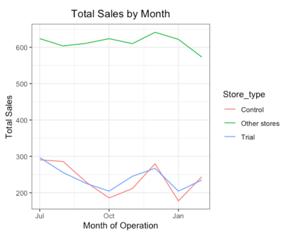
#### Now that we have found control store 233 for trial store 77, let’s check visually if the #### drivers are indeed similar in the period before the trial.
### sales
#### Visual checks on trends based on the drivers
trial_store <- 77
control_store <- 233
measureOverTimeSales <- as.data.table(measureOverTime)
pastSales <- measureOverTimeSales[, Store_type := ifelse(STORE_NBR == trial_store,
"Trial",ifelse(STORE_NBR == control_store,"Control", "Other stores"))][, totSales := mean(totSales),
by = c("YEARMONTH","Store_type")][, TransactionMonth := as.Date(paste(YEARMONTH %/%100, YEARMONTH %% 100, 1, sep = "‐"), "%Y‐%m‐%d")][YEARMONTH < 201903 , ]
### Visualize
ggplot(pastSales, aes(TransactionMonth, totSales, color = Store_type)) +
geom_line() +
labs(x = "Month of Operation", y= "Total Sales", title = "Total Sales by Month")
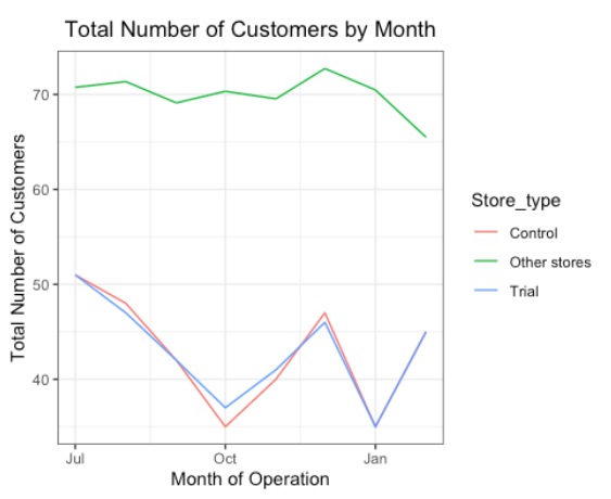
### customers
measureOverTimeCusts <- as.data.table(measureOverTime)
pastCustomers <- measureOverTimeCusts[, Store_type := ifelse(STORE_NBR == trial_store, "Trial", ifelse(STORE_NBR == control_store,"Control","Other stores"))][, numberCustomers := mean(nCustomers),
by = c("YEARMONTH","Store_type")][, TransactionMonth := as.Date(paste(YEARMONTH %/%100,
YEARMONTH %% 100, 1, sep = "‐"), "%Y‐%m‐%d")][YEARMONTH < 201903 ]
### Visualize
ggplot(pastCustomers, aes(TransactionMonth, numberCustomers, color = Store_type)) +
geom_line() + labs(x = "Month of Operation",
y = "Total Number of Customers",
title = "Total Number of Customers by Month")
### Assessment of trial
### The trial period goes from the start of February 2019 to April 2019. We now want to
### see if there has been an uplift in overall chip sales.
### We'll start with scaling the control store's sales to a level similar to control
### for any differences between the two stores outside of the trial period.
#### Scale pre-trial control sales to match pre-trial trial store sales
trial_store <- 77
control_store <- 233
preTrialMeasures <- as.data.table(preTrialMeasures)
scalingFactorForControlSales <- preTrialMeasures[STORE_NBR == trial_store & YEARMONTH < 201902, sum(totSales)]/preTrialMeasures[STORE_NBR == control_store &YEARMONTH < 201902, sum(totSales)]
#### Apply the scaling factor
measureOverTimeSales <- measureOverTime
measureOverTimeSales$controlSales <- measureOverTimeSales$totSales * scalingFactorForControlSales
scaledControlSales <- measureOverTimeSales[measureOverTimeSales$STORE_NBR == control_store, ]
### Now that we have comparable sales figures for the control store, we can calculate the
### percentage difference between the scaled control sales and the trial store's sales
### during the trial period.
measureOverTime <- as.data.table(measureOverTime)
percentageDiff <- merge(scaledControlSales[, c("YEARMONTH", "controlSales")],
measureOverTime[STORE_NBR == trial_store, c("totSales", "YEARMONTH")], by = "YEARMONTH")
percentageDiff$percentageDiff <- round(abs((percentageDiff$controlSales - percentageDiff$totSales)/percentageDiff$controlSales),3)
### Let's see if the difference is significant!
#### As our null hypothesis is that the trial period is the same as the pre-trial period,
### let's take the standard deviation based on the scaled percentage difference in the
### pre-trial period.
std <-subset(percentageDiff, YEARMONTH < 201902, select = c(YEARMONTH, percentageDiff))
stdDev <- sd(std$percentageDiff)
#### Note that there are 8 months in the pre-trial period
#### hence 8 - 1 = 7 degrees of freedom
degreesOfFreedom <- 7
#### We will test with a null hypothesis of there being 0 difference between trial and control ### stores.
### Calculate the t-values for the trial months. After that, find the 95th percentile of the
### t distribution with the appropriate degrees of freedom to check whether the hypothesis ### is statistically significant.
### Hint: The test statistic here is (x - u)/standard deviation
percentageDiff$t_value <- (percentageDiff$percentageDiff - 0)/stdDev
percentageDiff$TransactionMonth <- as.Date(paste(percentageDiff$YEARMONTH %/% 100, percentageDiff$YEARMONTH %% 100, 1, sep = "-"),"%Y-%m-%d")
percentageDiff <- percentageDiff %>% filter(YEARMONTH < 201905 & YEARMONTH > 201901)
#### find the 95th percentile of the t distribution with the appropriate degrees of freedom to ### check whether the hypothesis is statistically significant.
qt(0.95, df = degreesOfFreedom)
### We can observe that the t-value is much larger than the 95th percentile value of the
### t-distribution for March
### and April - i.e. the increase in sales in the trial store in March and April is
### statistically greater than in the control store.
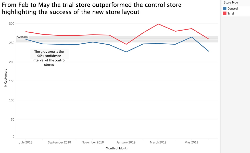
### Let's create a more visual version of this by plotting the sales of the control
### store, the sales of the trial stores and the 95th percentile value of sales of the control ### store.
measureOverTimeSales <- as.data.table(measureOverTime)
### Create new variables Store_type, totSales and TransactionMonth in the data table.
control_store <- 233
trial_store <- 77
pastSales <- measureOverTimeSales[, Store_type :=
ifelse(STORE_NBR ==trial_store, "Trial",
ifelse(STORE_NBR == control_store,"Control", "Other stores"))][, totSales :=mean(totSales), by = c("YEARMONTH","Store_type")][, TransactionMonth := as.Date(paste(YEARMONTH %/% 100, YEARMONTH %% 100, 1, sep = "‐"), "%Y‐%m‐%d")][Store_type %in% c("Trial", "Control"), ]
pastSales <- as.data.table(pastSales)
### Control Store 233 95th percentile
pastSales_Controls95 <- pastSales[ Store_type == "Control" ,
][, totSales := totSales * (1 + stdDev * 2)
][, Store_type := "Control 95th % confidence interval"]
### Control store 5th percentile
pastSales_Controls5 <- pastSales[Store_type == "Control" ,
][, totSales := totSales * (1 - stdDev * 2)
][, Store_type := "Control 5th % confidence interval"]
trialAssessment <- rbind(pastSales, pastSales_Controls95, pastSales_Controls5)
#### Plotting these in one nice graph
ggplot(trialAssessment, aes(TransactionMonth, totSales, color = Store_type)) +
geom_rect(data = trialAssessment[ YEARMONTH < 201905 & YEARMONTH > 201901 ,],aes(xmin = min(TransactionMonth), xmax = max(TransactionMonth), ymin = 0 , ymax = Inf, color = NULL), show.legend = FALSE) +
geom_line() +
labs(x = "Month of operation", y = "Total sales", title = "Total sales by month")
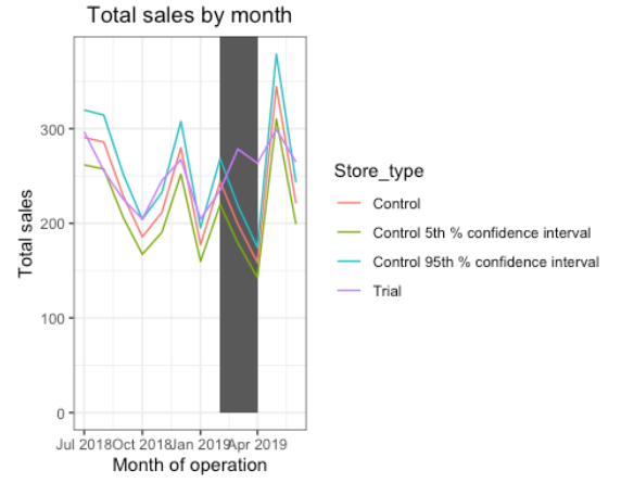
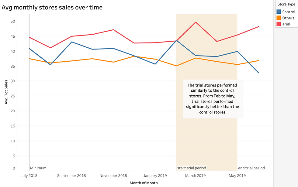
The results show that the trial in store 77 is significantly different to its control store in the trial period as the trial store performance lies outside the 5% to 95% confidence interval of the control store in two of the three trial months.
### Let's have a look at assessing this for number of customers as well.
preTrialMeasures <- as.data.table(preTrialMeasures)
scalingFactorForControlCusts <- preTrialMeasures[STORE_NBR == trial_store & YEARMONTH < 201902,sum(nCustomers)]/preTrialMeasures[STORE_NBR == control_store & YEARMONTH < 201902, sum(nCustomers)]
measureOverTimeCusts <- as.data.table(measureOverTime)
scaledControlCustomers <- measureOverTimeCusts[STORE_NBR == control_store, ][, controlCustomers := nCustomers * scalingFactorForControlCusts][,Store_type := ifelse(STORE_NBR == trial_store, "trial", ifelse(STORE_NBR == control_store,"control","Other Store"))]
### Calculate the % difference between scaled control sales and trial sales
percentageDiff <- merge(scaledControlCustomers[, c("YEARMONTH", "controlCustomers")],
measureOverTimeCusts[STORE_NBR == trial_store, c("nCustomers", "YEARMONTH")], by = "YEARMONTH")[ , percentageDiff := abs(controlCustomers - nCustomers)/controlCustomers]
#### As our null hypothesis is that the trial period is the same as the pre-trial period,
### let's take the standard deviation based on the scaled percentage difference in the
### pre-trial period
stdDev <- sd(percentageDiff[YEARMONTH < 201902 , percentageDiff])
degreesOfFreedom <- 7
#### Trial and control store number of customers
measureOverTimeCusts <- as.data.table(measureOverTime)
pastCustomers <- measureOverTimeCusts[, Store_type := ifelse(STORE_NBR == trial_store, "Trial",ifelse(STORE_NBR == control_store, "Control","Other stores"))][, nCusts := mean(nCustomers), by = c("YEARMONTH","Store_type")][, TransactionMonth := as.Date(paste(YEARMONTH %/% 100, YEARMONTH %% 100, 1, sep = "‐"), "%Y‐%m‐%d")][Store_type %in% c("Trial", "Control"), ]
### Control 95th percentile
pastCustomers_Control95 <- pastCustomers[Store_type == "Control",][, nCusts := nCusts * (1 + stdDev * 2)][, Store_type := "Control 95th % confidence interval"]
### Control 5th percentile
pastCustomers_Control5 <- pastCustomers[Store_type == "Control",][, nCusts := nCusts * (1 + stdDev * 2)][, Store_type := "Control 5th % confidence interval"]
trialAssessment <-rbind(pastCustomers,pastCustomers_Control95,pastCustomers_Control5)
### Visualize
ggplot(trialAssessment, aes(TransactionMonth, nCusts, color = Store_type)) +
geom_rect(data = trialAssessment[YEARMONTH < 201905 & YEARMONTH > 201901 , ],
aes(xmin = min(TransactionMonth), xmax = max(TransactionMonth),
ymin = 0, ymax = Inf, coor = NULL), show.legend = F) +
geom_line(aes(linetype = Store_type)) +
labs(x = "Month Of Operation",
y = "Total Number of Customers",
title = "Total Number of Customers by Month")
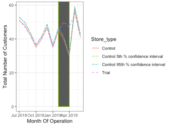
Results:
The results show that the trial in store 77 is significantly different to its control store in the trial period as the trial store performance lies outside the 5% to 95% confidence interval of the control store in two of the three trial months. We can check with the category manager if there were special deals in the trial store 77 that more people shopping at the store.
Skipping the repeat steps that we used for trial store 77 to each of the other two trial stores 88 and 86.
Conclusion:
We’ve found control stores 233, 155, 178 for trial stores 77, 86 and 88 respectively. The results for trial stores 77 and 88 during the trial period show a significant difference in at least two of the three trial months but this is not the case for trial store 86. Trial store 86 only shows one month sales higher. But the number of customers shows a significant difference in all three trial months. We can check with the client if the implementation of the trial was different in trial store 86.
Task three: Presentation
Create a presentation based on the analytics from the previous tasks. It is to provide insights and recommendations that the company's leaders can use when developing the strategic plan for the next half year.


Comments