Insurance Cross-selling Classification with XGboost-tree model
- gracecamc168
- Dec 30, 2020
- 5 min read
Updated: Jan 7, 2021
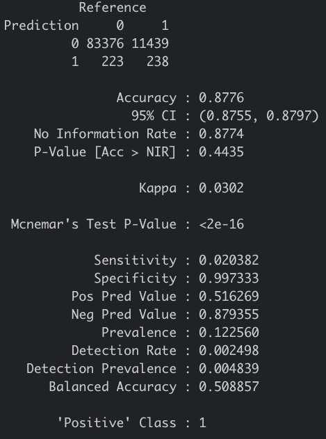
After submitting the project, I tried another objective model, which is XGboost with Tree. I wanted to know if tree based model is better than logistic model. The result is sort of right. But I would say if you don't have much time, this model will not be right for you. It took me more than four hours to finishing up tuning all the parameters, not to speak of fitting it back to the model. If you don't initially select the right parameters to tune like me, then it would definitely take you much more time than four hours. But I still think that it is good to try more models with XGboost because it is such a powerful model to, specially, deal with a complex dataset like if you have many variables in the dataset. One of the disadvantages of XGboost with tree based model is time consuming because there are many, like seven parameters, to be tuned. Otherwise, tuning parameters is the optimal choice. The overall accuracy of this model is 85%, which is a bit less than the GLM XGboost model that I used for my final submission of this project. The sensitivity rate of this tree-based model is 40%, meaning 60% of customers in reality are miss-labeled as purchasing the insurance when they are not, and 40% of customers are correctly labeled as going to purchase.The specificity rate is 91%, suggesting 9% of customers in reality are miss-labeled as going to purchase the insurance and 91% are correctly labeled as not going to purchase. It seems that it is still far from perfect of this classification, because this dataset has somewhat imbalanced classes issue. Dealing with imbalanced classes is extremely difficult, though I tuned all the parameters. We need to put a lot of efforts to do resample, boosting and try many different powerful Machine Learning models. However, we can play around the thresholds by plotting the ROC curve to select the best cutoff value for your preference of the business problem. R is the programming language for this project.
Let's start.
This dataset is the same one as I mentioned to my last Insurance post. You can download it from Kaggle(https://www.kaggle.com/anmolkumar/health-insurance-cross-sell-prediction). This is actually used as a competition. And I guess this is why they use it as a competition because of its difficulty. I will skip the EDA part because I did to my last post. If you are interested in, you can free to check out my last post. For this model, I will use tidymodel, which is inspired by Julia Silge, a great Data Scientist & Software Engineer.
library(tidyverse)
library(tidymodels)
library(caret)
library(xgboost)
# read the file and take a look of it
insurance <- read.csv("train.csv")
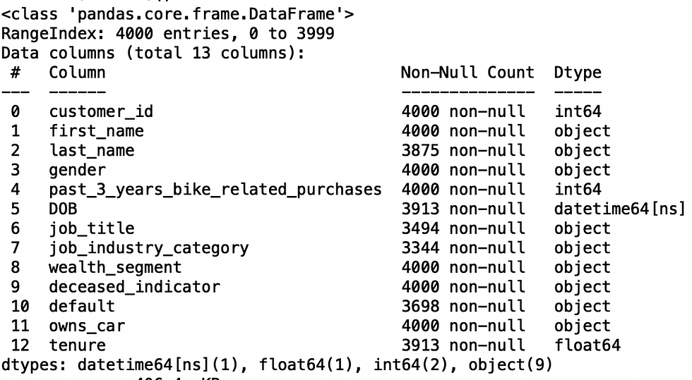
glimpse(insurance)
sum(!complete.cases(insurance)) # no missing values in this dataset
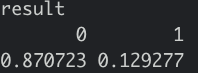
prop.table(table(insurance$Response)) # imbalanced classes

# convert the categorical variables to numeric because xgboost only works with
# numerical data
insurance$Gender <- ifelse(insurance$Gender == "Female", 0,1)
insurance$Vehicle_Damage <- ifelse(insurance$Vehicle_Damage == "Yes",1,0)
insurance$Vehicle_Age <- factor(insurance$Vehicle_Age,
c("< 1 Year","1-2 Year","> 2 Years"),
labels = c(1,2,3))
insurance$Vehicle_Age <- as.numeric(insurance$Vehicle_Age)
insurance$Response <- as.factor(insurance$Response)
# set the dataset into training and testing data as 75/25 ratio
set.seed(123)
split <- initial_split(insurance, strata = Response)
train <- training(split)
test <- testing(split)
# remove "id" variable because it is not significant
train <- train[ ,-1]
# tuning the best 6 parameters
xgb_spec <- boost_tree(
trees = 1000,# The number of trees contained in the ensemble
mtry = tune(), # The number of predictors that will be randomly sampled
# at each split when creating the tree models.
tree_depth = tune(), #The maximum depth of the tree (i.e. number of splits).
min_n = tune(), # The minimum number of data points in a node that is required
# for the node to be split further.
loss_reduction = tune(),# The reduction in the loss function required to split further.
sample_size = tune(), #The amount of data exposed to the fitting routine
learn_rate = tune()) %>% #The rate at which the boosting algorithm adapts from iteration-to-iteration.
set_engine("xgboost") %>%
set_mode("classification")
# if we use grid_regular function, it will take long time, so we use
# use grid_latin_hypercube function to tune these parameters
xgb.grid <- grid_latin_hypercube(
finalize(mtry(),train), # notice that we had to treat mtry() differently
# because it depends on the actual number of predictors in the data.
min_n(),
tree_depth(),
learn_rate(),
loss_reduction(),
sample_size = sample_prop(),# it should be a proportion, not actual numbers
size = 30 # 30 models will be trained
)
# create a workflow to put the formula and model together
xgb_wf <- workflow() %>%
add_formula(Response ~.) %>%
add_model(xgb_spec)
# 5-fold cross validation
five_fold <- vfold_cv(train,strata=Response ,v =5)
# you can try more, like 10 folds, but it definitely will take much more time, like six-eight hours.
# tune our parametrs
doParallel::registerDoParallel() # makes the process faster
set.seed(168)
xgb.tune <- tune_grid(
object=xgb_wf,# a workflow that contains model,
resamples = five_fold,
grid = xgb.grid, # the required parameters to be tuned
control = control_grid(save_pred = TRUE) # we can explore our predictions afterwards
)
# explore the tune
collect_metrics(xgb.tune )
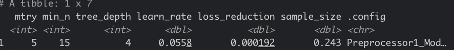
show_best(xgb.tune,"roc_auc") # check the best sets of parameters

# choose the best one
best_tune <- select_best(xgb.tune,"roc_auc")
best_tune
# let's finalize our workflow with the best parameters
final_xgb <- finalize_workflow(
xgb_wf,
best_tune)
# fit the model to the testing set
final_fit <- last_fit(final_xgb,split)
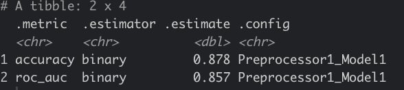
collect_metrics(final_fit )
# get the confusion matrix
final_fit %>%
collect_predictions() %>%
conf_mat(Response,.pred_class)
# recheck the proportion
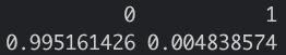
As we can see that the classification for 1(Purchase) is so poor, remember it was 12% from the orginal dataset. It is because we don't have enough Purchase class for this training.But this is actually better than the XGboost with GLM I tried.
# confusionMatrix in detail
prediction <- final_fit %>%
collect_predictions()
confusionMatrix(prediction$.pred_class,prediction$Response,positive="1")
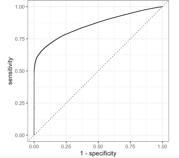
The ROC curve for Not Purchase class
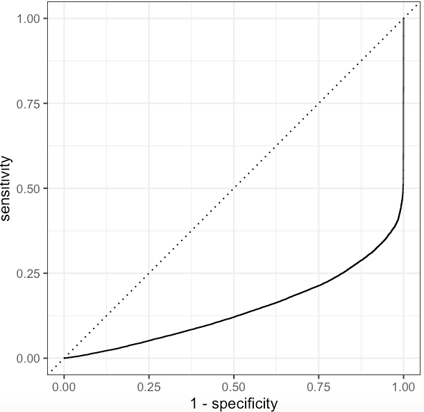
The ROC curve for Purchase class
As we can see, this is bad. But as I said, we can play around the threshold.
This model can be used if you just care about who is not going to purchase and want to receive low false positive rate.
Let's change the cutoff value to receive a different confusion matrix, because what if the company wants to sacrifice a bit marketing budget to get more customers who are going to purchase the insurance.
Let's set it to 0.33 as a cutoff value. We received a higher proportion of Purchase class and a new confusion matrix.

However, my teammate and I decided to choose a model that has a higher specificity rate and lower false positive rate, which is not in this case. We chose the model with 87.48% accuracy, 8.6 recall rate ,46% precision rate and 98% specificity rate. If you are interested in, you can check my last post for the XGboost logistic model. The code is similar to this one. Because we think not wasting marketing budget is more important in this cross-selling opportunity, compared to missing profit. If you think the same as us, you can definitely play around the thresholds to receive the similar performance matrix.
Lastly,I still want to receive a higher classification rate for Purchase class and low false positive rate without adjusting the threshold. If anyone knows, please let me know.


Comments